Tutorial 5: Recomendation Systems

I. CONTENT FILTERING

A. Item Profile

We start with a set of item characteristics. In our example we used whether the movie had Arnold Schwarzenegger, Julia Roberts as well as some measure of surprise in the script.

row_names<-c("AS", "JR", "surprise")
col_names<-c("PW", "TR", "EB", "T2", "P")

item <- matrix( c(0,   1,   0,   1, 1,
                                    1,   0,   1,   0, 0,                       
                                  0.1, 0.4, 0.1, 0, 0.1),
                                byrow = TRUE, nrow = 3, ncol = 5,
                                dimnames = list(row_names, col_names))
item %>% 
  kbl() %>%
  kable_styling()

	PW	TR	EB	T2	P
AS	0.0	1.0	0.0	1	1.0
JR	1.0	0.0	1.0	0	0.0
surprise	0.1	0.4	0.1	0	0.1

We also have Adam’s ratings of the items. We normalize them so that it is above/below his average rating.

rating <- matrix(c(3,1,5,2,4),nrow=1,ncol=5)
rating_m <- rating-mean(rating)

rating_m %>% 
  kbl() %>%
  kable_styling()

0

-2

2

-1

1

B. User Profile

To create the user profile, we need to see how much the users ratings change with the characteristics. The following tells us how much ratings change with attributes:

# t() means taking the transpose of a matrix, M'
user <- item %*% t(rating_m) / rowSums(item) ## This is the FORMULA in slides
user %>% 
  kbl() %>%
  kable_styling()

AS	-0.667
JR	1.000
surprise	-0.714

C. Similarity Prediction

To make predictions, we calculate the similarity between the user’s characteristic preferences and the characteristics of the items. The closer these two are, the better the fit.

row_names <- c("AS", "JR", "surprise")
col_names <- c("TL", "NH")

new_item <- matrix(c(1,0,
              0,1,
              .1,0), byrow = TRUE, nrow = 3, ncol = 2, dimnames=list(row_names,col_names))
new_item %>% 
  kbl() %>%
  kable_styling()

	TL	NH
AS	1.0	0
JR	0.0	1
surprise	0.1	0

CS = t(new_item) %*% user / (sqrt(colSums(new_item^2))*sqrt(sum(user^2))) ## FORMULA in slides
CS %>% 
  kbl() %>%
  kable_styling() ## We recomend more Noting Hill, as is closer to 1.

TL	-0.525
NH	0.715

D. Other Example

Now, Consider the item and rating matrix below:

row_names<-c("Funny", "Romant", "Suspense", "Dark")
col_names<-c("Sharp Obj", "Arrested Dev", "Arbitrage", "Margin C", "Bojack", "Orphan B", "Hinterland")

item <- matrix(c(0,1,0,1,1,1,0,
                 1,1,0,0,1,0,0,
                 1,1,1,0,1,0,1,
                 1,0,1,1,0,1,1), 
               byrow = TRUE, nrow = 4, ncol = 7, dimnames=list(row_names,col_names))

item %>% 
  kbl() %>%
  kable_styling()

	Sharp Obj	Arrested Dev	Arbitrage	Margin C	Bojack	Orphan B	Hinterland
Funny	0	1	0	1	1	1	0
Romant	1	1	0	0	1	0	0
Suspense	1	1	1	0	1	0	1
Dark	1	0	1	1	0	1	1

rating <- matrix(c(4,3,4,5,3),nrow=1,ncol=5)
rating %>% 
  kbl() %>%
  kable_styling()

4

3

4

5

3

Calculate the cosine similarity for the 2 movies and decide which to recommend.

User Profile

user <- item[,1:5] %*% t(rating) / rowSums(item) ## This is the FORMULA in slides

user %>% 
  kbl() %>%
  kable_styling()

Funny	2.75
Romant	3.33
Suspense	2.80
Dark	2.60

II. COLLABORATIVE FILTERING

From lecture we gave an example of 7 users and 6 items. We are trying to predict whether to recommend Predator or Notting Hill to Adam based on his similarity with others.

row_names<-c("A", "B", "C", "D", "E", "F", "G")
col_names<-c("PW", "TR", "EB", "T2", "P", "NH")

util <- matrix(c(2,5,4,2,NA, NA,
              5,1,2,NA,1,NA,
              5,5,5,5,5,5,
              2,5,NA,3,NA,NA,
              5,4,5,3,NA,5,
              1,5,NA,NA,NA,1,
              2,NA,5,NA,5,NA),byrow = TRUE, nrow = 7, ncol = 6, dimnames=list(row_names,col_names))
util %>% 
  kbl() %>%
  kable_styling()

	PW	TR	EB	T2	P	NH
A	2	5	4	2	NA	NA
B	5	1	2	NA	1	NA
C	5	5	5	5	5	5
D	2	5	NA	3	NA	NA
E	5	4	5	3	NA	5
F	1	5	NA	NA	NA	1
G	2	NA	5	NA	5	NA

User Based

Let’s take a look at user-based collaborative filtering. We’ll use simple correlations between users to see who is more similar to A.

cor(t(util), use="pairwise.complete.obs") %>% 
  kbl() %>%
  kable_styling()

## Warning in cor(t(util), use = "pairwise.complete.obs"): the standard deviation is zero

	A	B	C	D	E	F	G
A	1.000	-0.996	NA	0.945	0.174	1	1.000
B	-0.996	1.000	NA	-1.000	0.693	-1	-0.971
C	NA	NA	NA	NA	NA	NA	NA
D	0.945	-1.000	NA	1.000	-0.327	1	NA
E	0.174	0.693	NA	-0.327	1.000	-1	NA
F	1.000	-1.000	NA	1.000	-1.000	1	NA
G	1.000	-0.971	NA	NA	NA	NA	1.000

From this we see that only B, F and G are relevant: We focus only on the 3 most similar customers, B F and G.

m <- cor(t(util), use="pairwise.complete.obs") # re-run the correlation matrix

## Warning in cor(t(util), use = "pairwise.complete.obs"): the standard deviation is zero

# The relevant row
m[row=c("B","F","G"), col=c("A")] %>% 
  kbl() %>%
  kable_styling()

	x
B	-0.996
F	1.000
G	1.000

We normalize the ratings and multiply the correlations by their ratings of the movies in question, P and NH. Then we average to get the predicted ratings of Adam.

util_n <- util - rowMeans(util, na.rm=TRUE) #normalize

## Multiply the correlations by their ratings of the movies in question, P and N
predm <- m[row=c("B","F","G"),col=c("A")]*util_n[row=c("B","F","G"), col=c("P","NH")]
## Take the average
pred <- colMeans(predm, na.rm=TRUE)
pred %>% 
  kbl() %>%
  kable_styling()

	x
P	1.12
NH	-1.33

Adam’s ratings would be 1.122 higher than average for P and -1.333 for NH.

Item Based

Now for the item based filtering. We do the correlations across columns instead of rows.

m <- cor(util, use="pairwise.complete.obs")

Focus on last two columns. We focus on the movies that have either perfect positive or negative correlation. For P that is TR and EB, for NH that is PW.

m <- m[row=c("PW", "TR","EB"), col=c("P", "NH")]

# make NA anything less than 1
m[abs(m)<1] <- NA
m %>% 
  kbl() %>%
  kable_styling()

	P	NH
PW	NA	1
TR	1	NA
EB	1	NA

The prediction is the product of the correlation between the target movie and the other movies and Adam’s normalized reviews for the other movies:

predm<-m*util_n[row=c("A"),col=c("PW", "TR","EB")]
predm %>% 
  kbl() %>%
  kable_styling()

	P	NH
PW	NA	-1.25
TR	1.75	NA
EB	0.75	NA

pred<-colMeans(predm, na.rm = TRUE)
pred %>% 
  kbl() %>%
  kable_styling()

	x
P	1.25
NH	-1.25

Adam’s ratings would be 1.25 higher than average for P and -1.25 than average for NH.

III. REAL DATA EXAMPLES

0. Data

data("MovieLense")
MovieLense

## 943 x 1664 rating matrix of class 'realRatingMatrix' with 99392 ratings.

#getRatingMatrix(MovieLense)[1:10,1:5]
as(MovieLense, "matrix")[1:10, 1:5]

##    Toy Story (1995) GoldenEye (1995) Four Rooms (1995) Get Shorty (1995) Copycat (1995)
## 1                 5                3                 4                 3              3
## 2                 4               NA                NA                NA             NA
## 3                NA               NA                NA                NA             NA
## 4                NA               NA                NA                NA             NA
## 5                 4                3                NA                NA             NA
## 6                 4               NA                NA                NA             NA
## 7                NA               NA                NA                 5             NA
## 8                NA               NA                NA                NA             NA
## 9                NA               NA                NA                NA             NA
## 10                4               NA                NA                 4             NA

test <- as(MovieLense, "matrix")[1:10,]
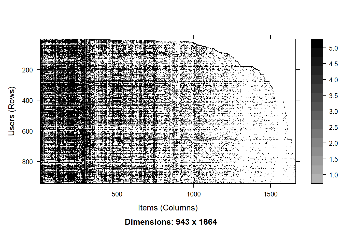
image(MovieLense)

count <- colCounts(MovieLense)
head(sort(count, decreasing = TRUE))

##            Star Wars (1977)              Contact (1997)                Fargo (1996) 
##                         583                         509                         508 
##   Return of the Jedi (1983)            Liar Liar (1997) English Patient, The (1996) 
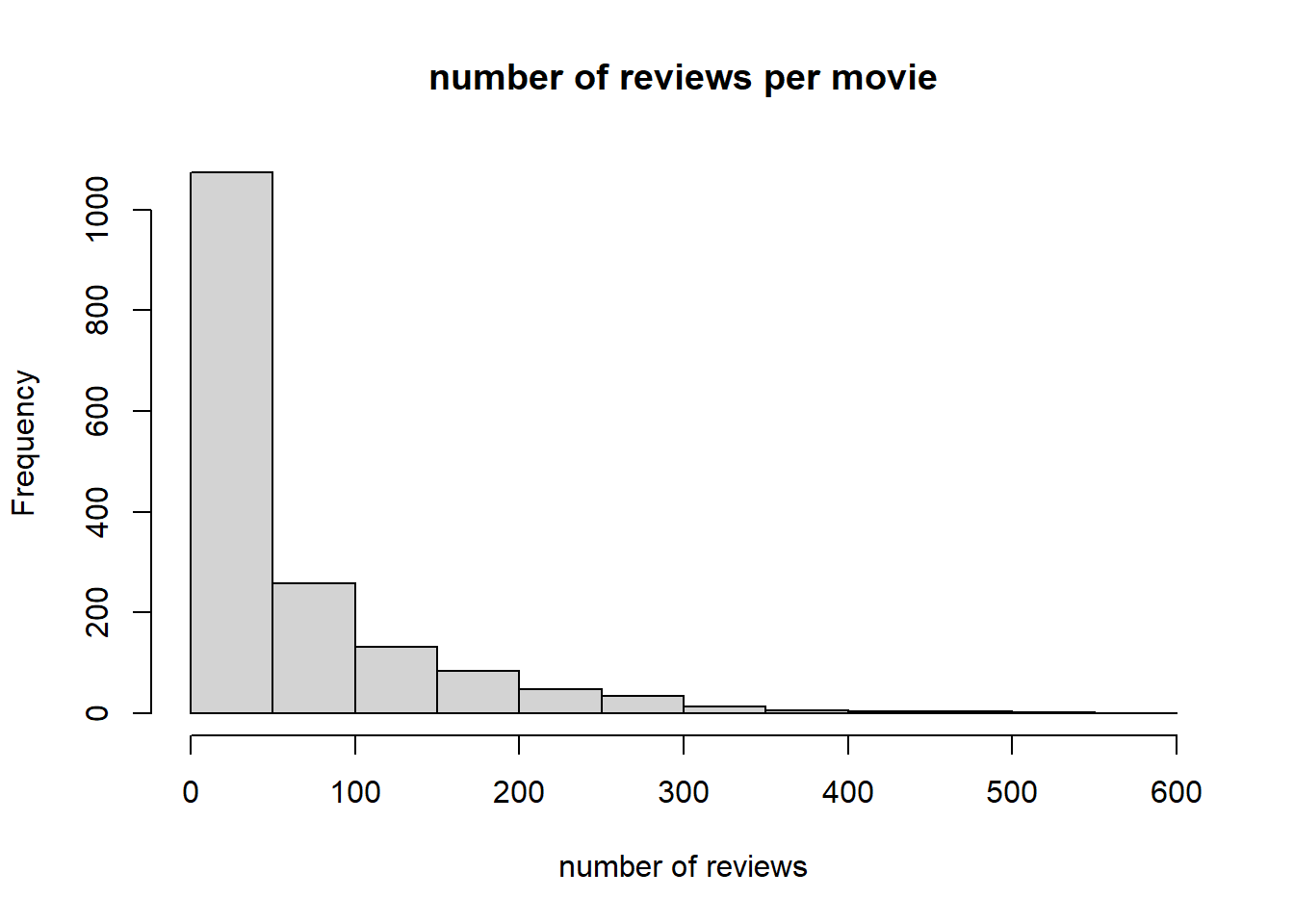
##                         507                         485                         481

hist(colCounts(MovieLense), xlab="number of reviews", main = "number of reviews per movie")

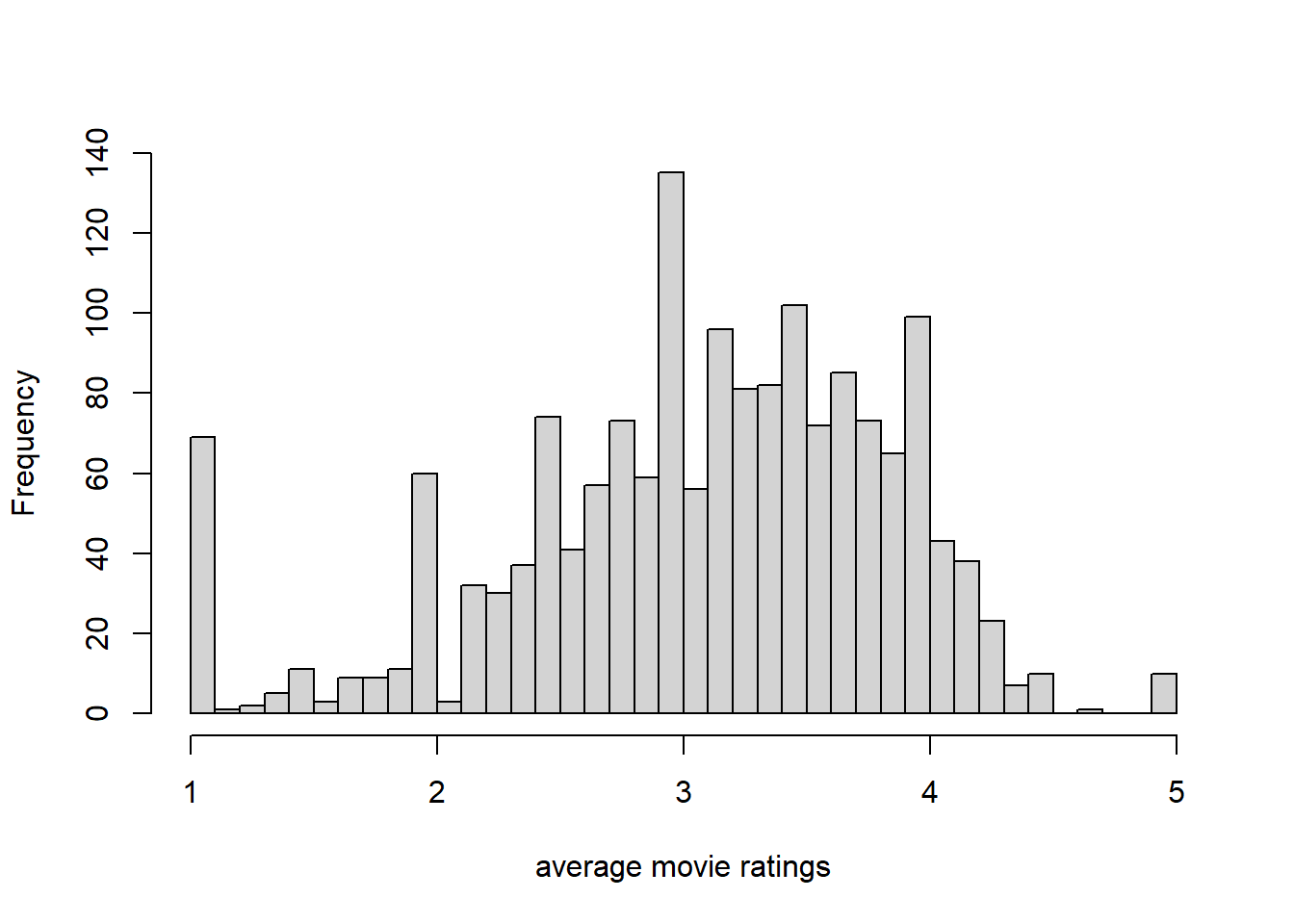
hist(colMeans(MovieLense), xlab="average movie ratings", main="", breaks=50)

1. Content Filtering

A. Build Item Profile

There are a bunch of meta-characteristics available. We’ll use the genres: from unknown to Western as our item characteristics.

head(MovieLenseMeta)

##                                                  title year
## 1                                     Toy Story (1995) 1995
## 2                                     GoldenEye (1995) 1995
## 3                                    Four Rooms (1995) 1995
## 4                                    Get Shorty (1995) 1995
## 5                                       Copycat (1995) 1995
## 6 Shanghai Triad (Yao a yao yao dao waipo qiao) (1995) 1995
##                                                            url unknown Action Adventure Animation
## 1        http://us.imdb.com/M/title-exact?Toy%20Story%20(1995)       0      0         0         1
## 2          http://us.imdb.com/M/title-exact?GoldenEye%20(1995)       0      1         1         0
## 3       http://us.imdb.com/M/title-exact?Four%20Rooms%20(1995)       0      0         0         0
## 4       http://us.imdb.com/M/title-exact?Get%20Shorty%20(1995)       0      1         0         0
## 5            http://us.imdb.com/M/title-exact?Copycat%20(1995)       0      0         0         0
## 6 http://us.imdb.com/Title?Yao+a+yao+yao+dao+waipo+qiao+(1995)       0      0         0         0
##   Children's Comedy Crime Documentary Drama Fantasy Film-Noir Horror Musical Mystery Romance Sci-Fi
## 1          1      1     0           0     0       0         0      0       0       0       0      0
## 2          0      0     0           0     0       0         0      0       0       0       0      0
## 3          0      0     0           0     0       0         0      0       0       0       0      0
## 4          0      1     0           0     1       0         0      0       0       0       0      0
## 5          0      0     1           0     1       0         0      0       0       0       0      0
## 6          0      0     0           0     1       0         0      0       0       0       0      0
##   Thriller War Western
## 1        0   0       0
## 2        1   0       0
## 3        1   0       0
## 4        0   0       0
## 5        1   0       0
## 6        0   0       0

item <- as.matrix(subset(MovieLenseMeta, select = -c(title, year, url)))

B. Build User Profile

We’ll take user 1 as our “Adam”, our user on which to build our content filtering system. We normalize his ratings by subtracting off the mean. We create an index, non_miss of the ratings he gives.

rating <- as(MovieLense, "matrix")[1,]

rating_m <- rating-mean(rating,na.rm=TRUE) ## normalize

non_miss <- !is.na(rating_m)
miss <- is.na(rating_m)

We calculate his user profile using the formula (slides). Only difference is that the item matrix is the opposite from the above example: movies are rows and attributes are columns.

So we change the matrix multiplication: transpose item matrix and take column sums rather than row sums.

user <- (t(item[non_miss,]) %*% rating_m[non_miss]) / colSums(item[non_miss, ])
user

##                 [,1]
## unknown      0.39483
## Action      -0.27183
## Adventure   -0.67659
## Animation   -0.27183
## Children's  -1.40517
## Comedy      -0.13264
## Crime       -0.16517
## Documentary  1.19483
## Drama        0.30993
## Fantasy     -0.10517
## Film-Noir    1.39483
## Horror      -0.14363
## Musical     -0.68209
## Mystery     -0.00517
## Romance      0.30181
## Sci-Fi       0.39483
## Thriller     0.01022
## War          0.07483
## Western      0.06150

C. Similarity Prediction

We take all of the movies he/she has not seen, and make our cosine similarity predictions on them.

names <- as.matrix(subset(MovieLenseMeta, select = c(title)))
new_item <- item[miss,]
new_names <- names[miss,]

We apply the formula:

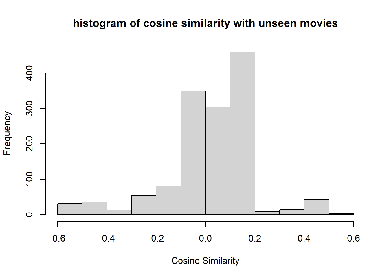
CS = (new_item) %*% user / (sqrt(rowSums(new_item^2))*sqrt(sum(user^2)))
hist(CS, main = "histogram of cosine similarity with unseen movies", xlab="Cosine Similarity")

The top 6 movies predicted (of the 1393 not rated movies) are:

new_names[head(order(CS, decreasing = TRUE))]

##                                                           488 
##                                         "Sunset Blvd. (1950)" 
##                                                          1476 
##                                             "Raw Deal (1948)" 
##                                                          1582 
##                                                "T-Men (1947)" 
##                                                           320 
## "Paradise Lost: The Child Murders at Robin Hood Hills (1996)" 
##                                                           360 
##                                           "Wonderland (1997)" 
##                                                           634 
##                    "Microcosmos: Le peuple de l'herbe (1996)"

2. Non-Personalized Recommendations: Popularity

Popular normalizes the ratings by user, and takes the average across users. It doesn’t recommend something to someone who has already rated it. But it starts at the top of the list and goes down.

row_names<-c("A", "B", "C", "D", "E", "F", "G")
col_names<-c("PW", "TR", "EB", "T2", "P", "NH")

util <- matrix(c(2,5,4,2,NA, NA,
              5,1,2,NA,1,NA,
              5,5,5,5,5,5,
              2,5,NA,3,NA,NA,
              5,4,5,3,NA,5,
              1,5,NA,NA,NA,1,
              2,NA,5,NA,5,NA),byrow = TRUE, nrow = 7, ncol = 6, dimnames=list(row_names,col_names))
util %>% 
  kbl() %>%
  kable_styling()

	PW	TR	EB	T2	P	NH
A	2	5	4	2	NA	NA
B	5	1	2	NA	1	NA
C	5	5	5	5	5	5
D	2	5	NA	3	NA	NA
E	5	4	5	3	NA	5
F	1	5	NA	NA	NA	1
G	2	NA	5	NA	5	NA

util_n <-util-rowMeans(util, na.rm=TRUE)

In our example above in the collaborative filtering part, it would make TR the first, EB the second, etc. If someone had already watched TR, the first recommendation would be EB, then P, etc.

colMeans(util_n,na.rm = TRUE) %>% 
  kbl() %>%
  kable_styling()

	x
PW	-0.367
TR	0.739
EB	0.420
T2	-0.746
P	-0.083
NH	-0.244

test<- as(util, "realRatingMatrix")
test_recom<-Recommender(test, method = "POPULAR")
test_recom@model$topN@items

## [[1]]
## [1] 2 3 5 6 1 4

test_pred<-predict(test_recom, test[1,],type="ratings")

as(test_pred,"matrix") %>% 
  kbl() %>%
  kable_styling()

	PW	TR	EB	T2	P	NH
A	NA	NA	NA	NA	3.17	3.01

Adam’s average review is 3.25. The average rating of P is -0.083 compared to the average. Hence the prediction of the popular model is these two quantities added, 3.167.

3. Collaborative Filtering

0. MovieLense “Method

set.seed(19103)
es <- evaluationScheme(MovieLense, 
  method="split", train=0.9, given=15)

## as(<dgCMatrix>, "dgTMatrix") is deprecated since Matrix 1.5-0; do as(., "TsparseMatrix") instead

es

## Evaluation scheme with 15 items given
## Method: 'split' with 1 run(s).
## Training set proportion: 0.900
## Good ratings: NA
## Data set: 943 x 1664 rating matrix of class 'realRatingMatrix' with 99392 ratings.

train <- getData(es, "train"); train

## 848 x 1664 rating matrix of class 'realRatingMatrix' with 90673 ratings.

test_known <- getData(es, "known"); test_known

## 95 x 1664 rating matrix of class 'realRatingMatrix' with 1425 ratings.

test_unknown <- getData(es, "unknown"); test_unknown

## 95 x 1664 rating matrix of class 'realRatingMatrix' with 7294 ratings.

popular <-Recommender(train, "POPULAR")
## create predictions for the test users using known ratings
pred_pop <- predict(popular, test_known, type="ratings"); pred_pop

## 95 x 1664 rating matrix of class 'realRatingMatrix' with 155897 ratings.

## evaluate recommendations on "unknown" ratings
acc_pop <- calcPredictionAccuracy(pred_pop, test_unknown);
as(acc_pop,"matrix") %>% 
  kbl() %>%
  kable_styling()

RMSE	0.989
MSE	0.977
MAE	0.780

as(test_unknown, "matrix")[1:8,1:5]

##    Toy Story (1995) GoldenEye (1995) Four Rooms (1995) Get Shorty (1995) Copycat (1995)
## 10                4               NA                NA                 4             NA
## 35               NA               NA                NA                NA             NA
## 53               NA               NA                NA                NA             NA
## 65                3               NA                NA                NA             NA
## 66                3               NA                NA                NA             NA
## 78               NA               NA                NA                NA             NA
## 79                4               NA                NA                NA             NA
## 94                4               NA                NA                 4             NA

as(pred_pop, "matrix")[1:8,1:5]

##    Toy Story (1995) GoldenEye (1995) Four Rooms (1995) Get Shorty (1995) Copycat (1995)
## 10             4.43             3.83              3.72              4.09           3.99
## 35             3.56             2.97              2.85              3.22           3.12
## 53             4.03             3.43              3.32              3.69           3.59
## 65             4.43             3.83              3.72              4.09           3.99
## 66             3.16             2.57              2.45              2.82           2.72
## 78             3.56             2.97              2.85              3.22           3.12
## 79             4.23             3.63              3.52              3.89           3.79
## 94             3.56             2.97              2.85              3.22           3.12

A. User-Based

Now we’ll use user-based collaborative filtering. We’ll use (pearson) correlation to determine the similarity across users.

And we’ll use the 30 most similar users in making our recommendation.

UBCF <- Recommender(train, "UBCF",
                        param=list(method="pearson",nn=30))

## create predictions for the test users using known ratings
pred_ub <- predict(UBCF, test_known, type="ratings"); pred_ub

## 95 x 1664 rating matrix of class 'realRatingMatrix' with 75118 ratings.

## evaluate recommendations on "unknown" ratings
acc_ub <- calcPredictionAccuracy(pred_ub, test_unknown);
acc <- rbind(POP=acc_pop, UBCF = acc_ub); acc

##       RMSE   MSE  MAE
## POP  0.989 0.977 0.78
## UBCF 1.118 1.251 0.88

as(test_unknown, "matrix")[1:8,1:5]

##    Toy Story (1995) GoldenEye (1995) Four Rooms (1995) Get Shorty (1995) Copycat (1995)
## 10                4               NA                NA                 4             NA
## 35               NA               NA                NA                NA             NA
## 53               NA               NA                NA                NA             NA
## 65                3               NA                NA                NA             NA
## 66                3               NA                NA                NA             NA
## 78               NA               NA                NA                NA             NA
## 79                4               NA                NA                NA             NA
## 94                4               NA                NA                 4             NA

as(pred_ub, "matrix")[1:8,1:5]

##    Toy Story (1995) GoldenEye (1995) Four Rooms (1995) Get Shorty (1995) Copycat (1995)
## 10             4.47             3.80              3.88              4.38           4.22
## 35             3.43             2.75              1.74              3.45           3.13
## 53             4.10               NA                NA              3.70           2.50
## 65             3.43               NA              4.39                NA           4.21
## 66             3.25             2.51                NA              3.55           4.21
## 78             3.85             2.69                NA              3.47           2.96
## 79             4.22             3.72              5.09              3.91           3.29
## 94             3.66             2.56              2.22              2.92           2.88

UBCF has higher error metrics than popularity, indicating worse fit.

B. Item-Based

Here we use item-based collaborative filtering, using peason correlation to determine similarity across items. And we use the 30 most similiar items.

IBCF <- Recommender(train, "IBCF",
                        param=list(method="pearson",k=30))

pred_ib <- predict(IBCF, test_known, type="ratings")

acc_ib <- calcPredictionAccuracy(pred_ib, test_unknown) 

acc <- rbind(POP=acc_pop, UBCF = acc_ub, IBCF = acc_ib); acc

##       RMSE   MSE  MAE
## POP  0.989 0.977 0.78
## UBCF 1.118 1.251 0.88
## IBCF 1.507 2.271 1.16

Note the error metric is yet worse for IBCF.