Quiz 6: CLV - Contractual Settings
Daniel Redel
2023-01-26
Question 1
Consider Netflix. A month-long subscription from a customer generates a profit flow of 10 per month, and they use a 0.008 discount rate. Below is a cohort of subscribers who all began their subscription in January 2020: 1000 initially joined; a month later 631 of them did not cancel, etc.
active_cust=c(1000,
              631,
              468,
              382,
              326,
              289,
              262,
              241,
              223,
              207,
              194)

cbind(0:10,active_cust) %>%
  kbl() %>%
kable_styling()| active_cust | |
|---|---|
| 0 | 1000 |
| 1 | 631 |
| 2 | 468 |
| 3 | 382 |
| 4 | 326 |
| 5 | 289 |
| 6 | 262 |
| 7 | 241 |
| 8 | 223 |
| 9 | 207 |
| 10 | 194 |
What is the actual retention rate and actual survival function at 10 months since joining?
Provide your answers with a dot and three decimals (e.g. 0.234)
Survivor Function:
S <- active_cust/active_cust[1]
S
## [1] 1.000 0.631 0.468 0.382 0.326 0.289 0.262 0.241 0.223 0.207 0.194Retention Rate:
r <- S[2:11]/S[1:10]
r
## [1] 0.631 0.742 0.816 0.853 0.887 0.907 0.920 0.925 0.928 0.937Final Data:
cbind(0:10, S, c(NA,r)) %>%
  kbl() %>%
kable_styling()| S | ||
|---|---|---|
| 0 | 1.000 | NA |
| 1 | 0.631 | 0.631 |
| 2 | 0.468 | 0.742 |
| 3 | 0.382 | 0.816 |
| 4 | 0.326 | 0.853 |
| 5 | 0.289 | 0.887 |
| 6 | 0.262 | 0.907 |
| 7 | 0.241 | 0.920 |
| 8 | 0.223 | 0.925 |
| 9 | 0.207 | 0.928 |
| 10 | 0.194 | 0.937 |
Question 2
Fit the Beta-Geometric model to the retention data using only data from the beginning until (and including) 4 months since joining. For your estimation use starting values a = 1 and b = 1.
What are the estimates of a and b?
Provide your answers with a dot and three decimals (e.g. 0.123)
Calibration Sample:
lost <- -diff(active_cust[1:5])
active <- active_cust[1:5][-1]
Likelihood Estimation:
loop.lik <- function(params) {
a <- params[1]
b <- params[2]

ll <- 0
for (i in 1:length(lost)) {
    ll <- ll+lost[i]*log(beta(a+1,b+i-1)/beta(a,b))
}
ll <- ll+active[i]*log(beta(a,b+i)/beta(a,b))
return(-ll)  #return the negative of the function to max. LL
}

#find parameters for a and b with optim
sBG <- optim(par=c(1,1),loop.lik)
a <- sBG$par[1]
b <- sBG$par[2]## a= 0.763 b= 1.29Question 3
Our holdout sample is everything after period 4.
How well does the model fit the data from period 5 onward? Make a graph. Use the model estimates to predict retention and survival function at 10 months since joining.
Provide your answers with a dot and three decimals (e.g. 0.234)
Retention Rate (Prediction):
r_sBG = function(a,b,t){
    (b+t-1)/(a+b+t-1)
}
# Prediction
t <- seq(1:10)
r_pred <- r_sBG(a,b,t)
par(mfrow=c(1,1))
plot(t, r_pred,ylab="retention rate",xlab="period",type="b", xaxt="none", ylim = c(.55,1))
lines(t, r, type="b", col="blue")
axis(1, seq(0,10,1))
legend('right',legend=c("sBG", "actual"),col=c("black","blue"), pch=c(1,1))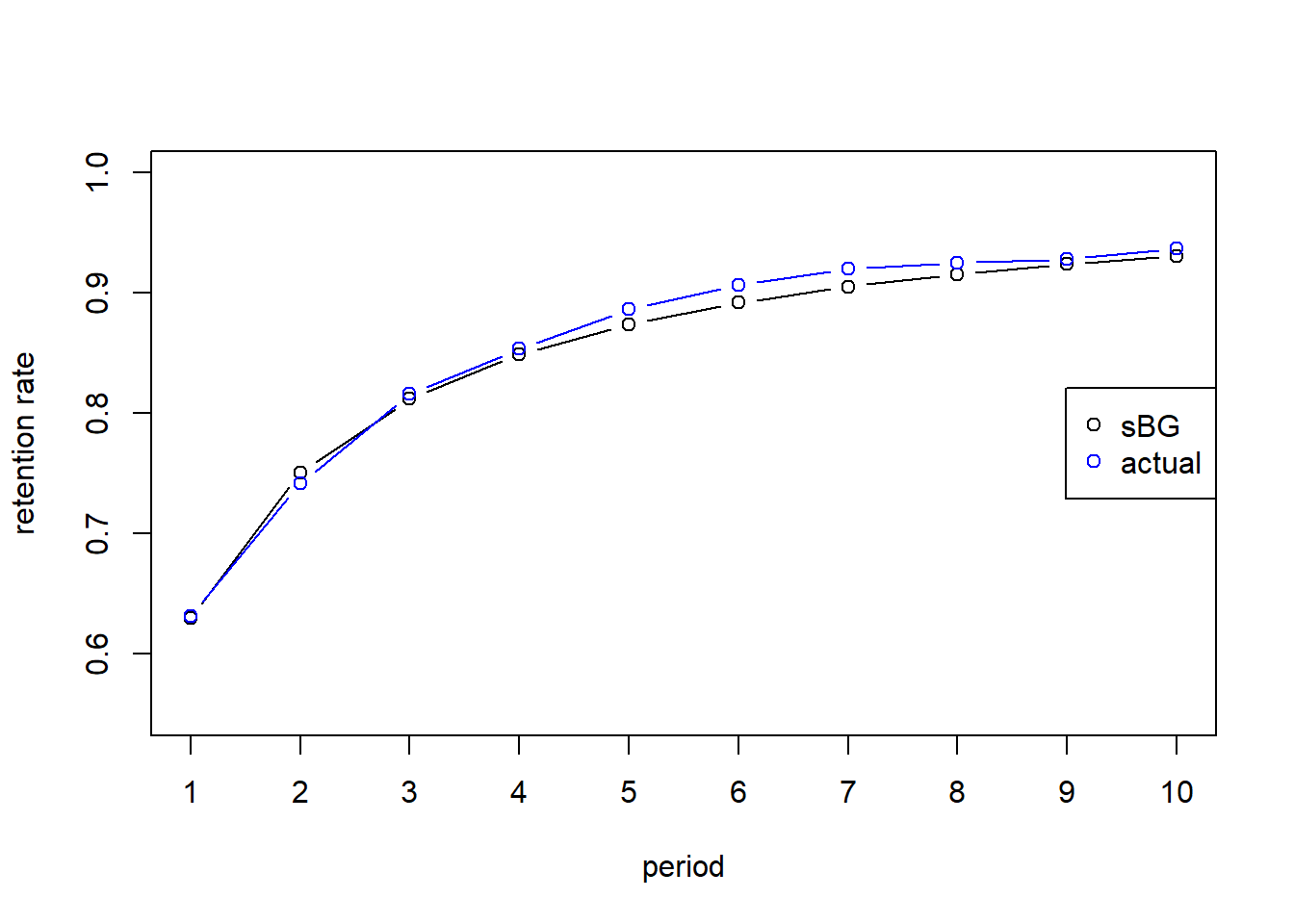
Survivor Function (Prediction):
S_pred <- c(1,cumprod(r_pred))
S_pred
## [1] 1.000 0.629 0.472 0.383 0.325 0.284 0.254 0.230 0.210 0.194 0.181par(mfrow=c(1,1))
plot(seq(0:10), S_pred, ylab="retention rate",xlab="period",type="b", xaxt="none", ylim = c(0,1))
lines(seq(0:10),S, type="b", col="blue")
axis(1, seq(0,10,1))
legend('right',legend=c("sBG", "geo", "actual"),col=c("black","red","blue"), pch=c(1,1))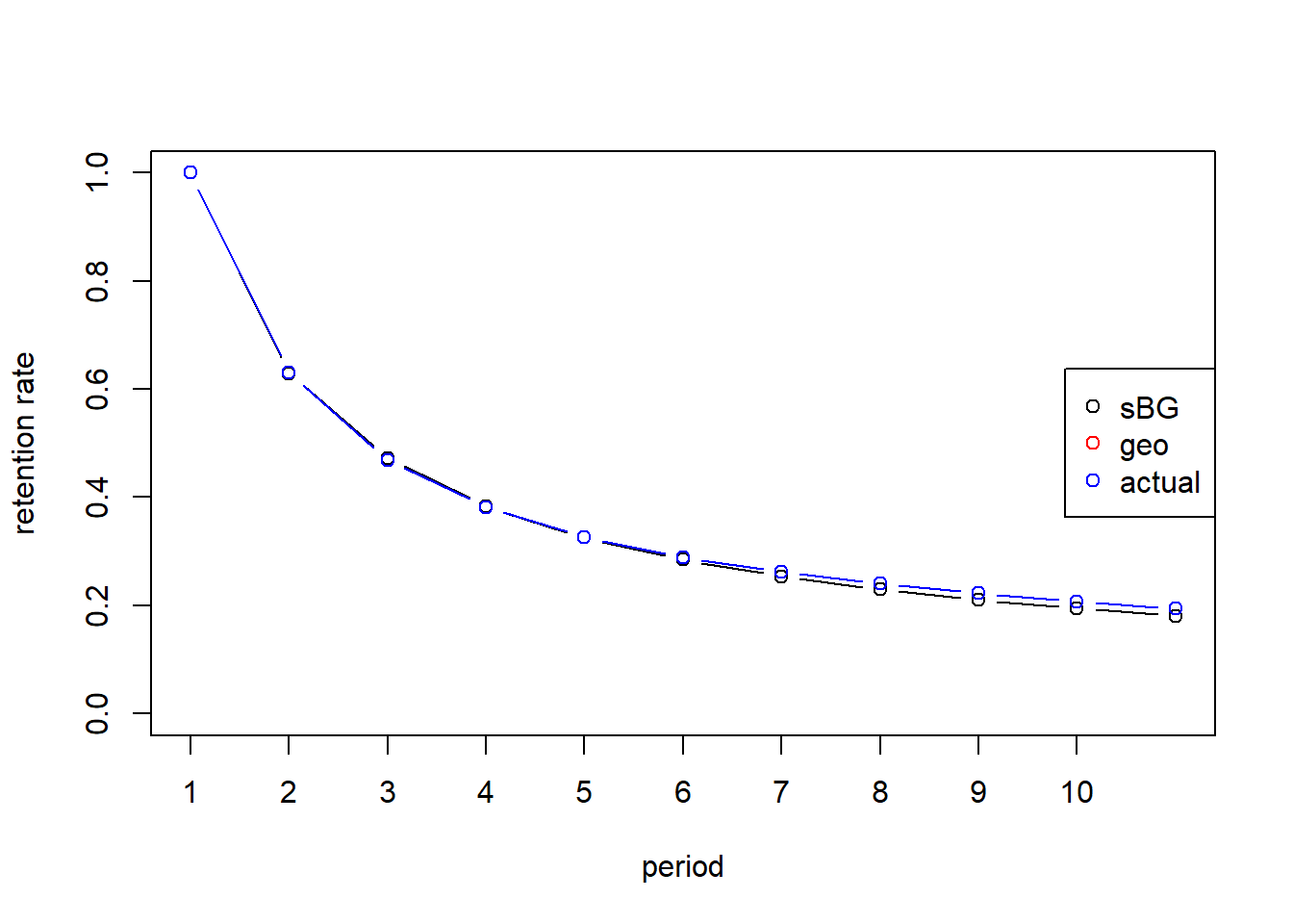
Question 4
Up to how much would Netflix pay to acquire a new customer with a value according to that implied by the model? Use 200 months in your calculation.
Round to the nearest whole number.
CLV:
d <- 0.008
m <- 10
t <- seq(1,200) # time periods
r_pred <- r_sBG(a,b,t) # predicted retention rate
S_pred <- c(1,cumprod(r_pred)[1:199])

dis <- 1/(1+d)^(t-1) # discount factor, first term is present so no discounting

CLV_sBG <- sum(m*S_pred*dis) # the sum of margin x survivor x discount factor
CLV_sBG
## [1] 90.1Question 5
Now calculate CLV using the geometric model that assumes a constant retention rate.
To estimate that constant rate, you can use the results of the BG model. The average retention rate in the population at time 0 is b/(a+b). Use that quantity as your estimate of the retention rate for the geometric model.
Give the whole number.
geoCLV<-function(p,m,d){
  m*(1+d)/(1+d-p)
}

p <- b/(a+b) # its B! not A
geo <- geoCLV(p, m, d) # use that estimate
round(geo,0)
## [1] 27Question 6
Back to the original BG coefficients.
What is the expected residual lifetime value of a customer who has renewed once, standing just before time 2, when he or she makes his or her second renewal decision?
Give the whole number.
RLV:
tau<-1

t<-seq(1,tau+200)
r_pred<-r_sBG(a,b,t)
S_pred<-cumprod(r_pred)
S_shift <- S_pred[(tau+1):length(S_pred)] # survival function from tau + 1 until T
dis <- 1/(1+d)^(t(1:200)-1) # discount rate
RLV_sBG<-sum(m*S_shift/S_pred[tau]*dis)
RLV_sBG## [1] 119