Assignment 4: Subset Selection, LASSO & Trees

Data Import:

bank <- read.csv('bank.csv', stringsAsFactors = TRUE)
bank <- bank[-c(1:3)]
n <- nrow(bank)

set.seed(19103)
sample <- sample(c(TRUE, FALSE), n, replace=TRUE, prob=c(0.7, 0.3))
bank.train <- bank[sample, ]
bank.holdout <- bank[!sample, ]

A bank wants to implement a proactive churn policy. They assemble a data set of past customers who either churned or stayed (were retained) along with several variables that can be used to predict this decision. This data set is called bank.csv. The churn variable is called Exited (1 churn, 0 not churn).

Question 1: What variable enters last in Forward Selection?

Use forward selection starting from an intercept-only model adding explanatory variables until the AIC minimum is reached or all 10 variables are added. What variable enters last?

Full Model, but without interaction terms (10 variables in total):

full <- glm(Exited ~ ., data=bank.train, family = "binomial")

summary(full)

## 
## Call:
## glm(formula = Exited ~ ., family = "binomial", data = bank.train)
## 
## Deviance Residuals: 
##    Min      1Q  Median      3Q     Max  
## -2.330  -0.665  -0.463  -0.274   2.969  
## 
## Coefficients:
##                       Estimate    Std. Error z value             Pr(>|z|)    
## (Intercept)      -3.2994976420  0.2910304887  -11.34 < 0.0000000000000002 ***
## CreditScore      -0.0006358323  0.0003335113   -1.91              0.05659 .  
## GeographyGermany  0.7481890738  0.0804480337    9.30 < 0.0000000000000002 ***
## GeographySpain    0.0089364591  0.0836470250    0.11              0.91492    
## GenderMale       -0.5503216618  0.0646080453   -8.52 < 0.0000000000000002 ***
## Age               0.0740294328  0.0030836019   24.01 < 0.0000000000000002 ***
## Tenure           -0.0216144137  0.0110427763   -1.96              0.05031 .  
## Balance           0.0000020672  0.0000006086    3.40              0.00068 ***
## NumOfProducts    -0.0870781223  0.0558204283   -1.56              0.11877    
## HasCrCard        -0.0685495618  0.0700553570   -0.98              0.32782    
## IsActiveMember   -1.0512041124  0.0683755435  -15.37 < 0.0000000000000002 ***
## EstimatedSalary  -0.0000000877  0.0000005603   -0.16              0.87565    
## ---
## Signif. codes:  0 '***' 0.001 '**' 0.01 '*' 0.05 '.' 0.1 ' ' 1
## 
## (Dispersion parameter for binomial family taken to be 1)
## 
##     Null deviance: 7161.0  on 7011  degrees of freedom
## Residual deviance: 6087.2  on 7000  degrees of freedom
## AIC: 6111
## 
## Number of Fisher Scoring iterations: 5

# intercept only
null <- glm(Exited ~ 1, data=bank.train, family = "binomial")

start_time <- Sys.time()
fwd.model=step(null, direction = 'forward', scope=formula(full), keep = function(model, aic) list(model = model, aic = aic))

## Start:  AIC=7163
## Exited ~ 1
## 
##                   Df Deviance  AIC
## + Age              1     6609 6613
## + Geography        2     6985 6991
## + IsActiveMember   1     7009 7013
## + Gender           1     7074 7078
## + Balance          1     7080 7084
## + NumOfProducts    1     7146 7150
## + CreditScore      1     7157 7161
## + Tenure           1     7159 7163
## <none>                   7161 7163
## + HasCrCard        1     7160 7164
## + EstimatedSalary  1     7161 7165
## 
## Step:  AIC=6613
## Exited ~ Age
## 
##                   Df Deviance  AIC
## + IsActiveMember   1     6344 6350
## + Geography        2     6444 6452
## + Gender           1     6526 6532
## + Balance          1     6536 6542
## + NumOfProducts    1     6600 6606
## + CreditScore      1     6605 6611
## + Tenure           1     6606 6612
## <none>                   6609 6613
## + HasCrCard        1     6609 6615
## + EstimatedSalary  1     6609 6615
## 
## Step:  AIC=6350
## Exited ~ Age + IsActiveMember
## 
##                   Df Deviance  AIC
## + Geography        2     6186 6196
## + Gender           1     6268 6276
## + Balance          1     6273 6281
## + NumOfProducts    1     6338 6346
## + Tenure           1     6340 6348
## + CreditScore      1     6341 6349
## <none>                   6344 6350
## + HasCrCard        1     6343 6351
## + EstimatedSalary  1     6344 6352
## 
## Step:  AIC=6196
## Exited ~ Age + IsActiveMember + Geography
## 
##                   Df Deviance  AIC
## + Gender           1     6114 6126
## + Balance          1     6172 6184
## + NumOfProducts    1     6180 6192
## + Tenure           1     6181 6193
## + CreditScore      1     6182 6194
## <none>                   6186 6196
## + HasCrCard        1     6185 6197
## + EstimatedSalary  1     6186 6198
## 
## Step:  AIC=6126
## Exited ~ Age + IsActiveMember + Geography + Gender
## 
##                   Df Deviance  AIC
## + Balance          1     6098 6112
## + NumOfProducts    1     6107 6121
## + Tenure           1     6110 6124
## + CreditScore      1     6111 6125
## <none>                   6114 6126
## + HasCrCard        1     6113 6127
## + EstimatedSalary  1     6114 6128
## 
## Step:  AIC=6112
## Exited ~ Age + IsActiveMember + Geography + Gender + Balance
## 
##                   Df Deviance  AIC
## + Tenure           1     6094 6110
## + CreditScore      1     6095 6111
## + NumOfProducts    1     6096 6112
## <none>                   6098 6112
## + HasCrCard        1     6097 6113
## + EstimatedSalary  1     6098 6114
## 
## Step:  AIC=6110
## Exited ~ Age + IsActiveMember + Geography + Gender + Balance + 
##     Tenure
## 
##                   Df Deviance  AIC
## + CreditScore      1     6091 6109
## + NumOfProducts    1     6092 6110
## <none>                   6094 6110
## + HasCrCard        1     6093 6111
## + EstimatedSalary  1     6094 6112
## 
## Step:  AIC=6109
## Exited ~ Age + IsActiveMember + Geography + Gender + Balance + 
##     Tenure + CreditScore
## 
##                   Df Deviance  AIC
## + NumOfProducts    1     6088 6108
## <none>                   6091 6109
## + HasCrCard        1     6090 6110
## + EstimatedSalary  1     6091 6111
## 
## Step:  AIC=6108
## Exited ~ Age + IsActiveMember + Geography + Gender + Balance + 
##     Tenure + CreditScore + NumOfProducts
## 
##                   Df Deviance  AIC
## <none>                   6088 6108
## + HasCrCard        1     6087 6109
## + EstimatedSalary  1     6088 6110

end_time<-Sys.time()
t=end_time-start_time

Here is the table showing the variables added per step.

fwd.model$anova

##               Step Df Deviance Resid. Df Resid. Dev  AIC
## 1                  NA       NA      7011       7161 7163
## 2            + Age -1   552.16      7010       6609 6613
## 3 + IsActiveMember -1   264.61      7009       6344 6350
## 4      + Geography -2   158.51      7007       6186 6196
## 5         + Gender -1    71.43      7006       6114 6126
## 6        + Balance -1    16.14      7005       6098 6112
## 7         + Tenure -1     3.92      7004       6094 6110
## 8    + CreditScore -1     3.61      7003       6091 6109
## 9  + NumOfProducts -1     2.45      7002       6088 6108

Question 2: How many variables (excluding the intercept) are in the final model?

Note not all coefficients were added.

## Forward Selection Model:  9

## Full Model:  11

Question 3: How many variables (excluding the intercept) are in this model?

Use the holdout data set to choose the right size model from the forward selection procedure. Choose the model with the largest Out Of Sample R2.

How many variables (excluding the intercept) are in this model?

set.seed(19103)
M <- dim(fwd.model$keep)[2]

OOS=data.frame(R2=rep(NA,M), rank=rep(NA, M))


## pred must be probabilities (0<pred<1) for binomial
deviance <- function(y, pred, family=c("gaussian","binomial")){
    family <- match.arg(family)
    if(family=="gaussian"){
      return( sum( (y-pred)^2 ) )
    }else{
      if(is.factor(y)) y <- as.numeric(y)>1
      return( -2*sum( y*log(pred) + (1-y)*log(1-pred) ) )
    }
  }

## get null devaince too, and return R2
  R2 <- function(y, pred, family=c("gaussian","binomial")){
  fam <- match.arg(family)
  if(fam=="binomial"){
    if(is.factor(y)){ y <- as.numeric(y)>1 }
  }
  dev <- deviance(y, pred, family=fam)
  dev0 <- deviance(y, mean(y), family=fam)
  return(1-dev/dev0)
  }  

for(k in 1:M){

pred = predict(fwd.model$keep[["model",k]], newdata=bank.holdout, type = "response")

OOS$R2[k]<-R2(y = bank.holdout$Exited,pred=pred, family="binomial")
OOS$rank[k]<-fwd.model$keep[["model",k]]$rank
  
  
}
ax=c(1:max(OOS$rank))
par(mai=c(.9,.8,.2,.2))
plot(x=OOS$rank, y = OOS$R2, type="b", ylab=expression(paste("Out-of-Sample R"^"2")), xlab="# of model parameters estimated (rank)", xaxt="n")
axis(1, at=ax, labels=ax)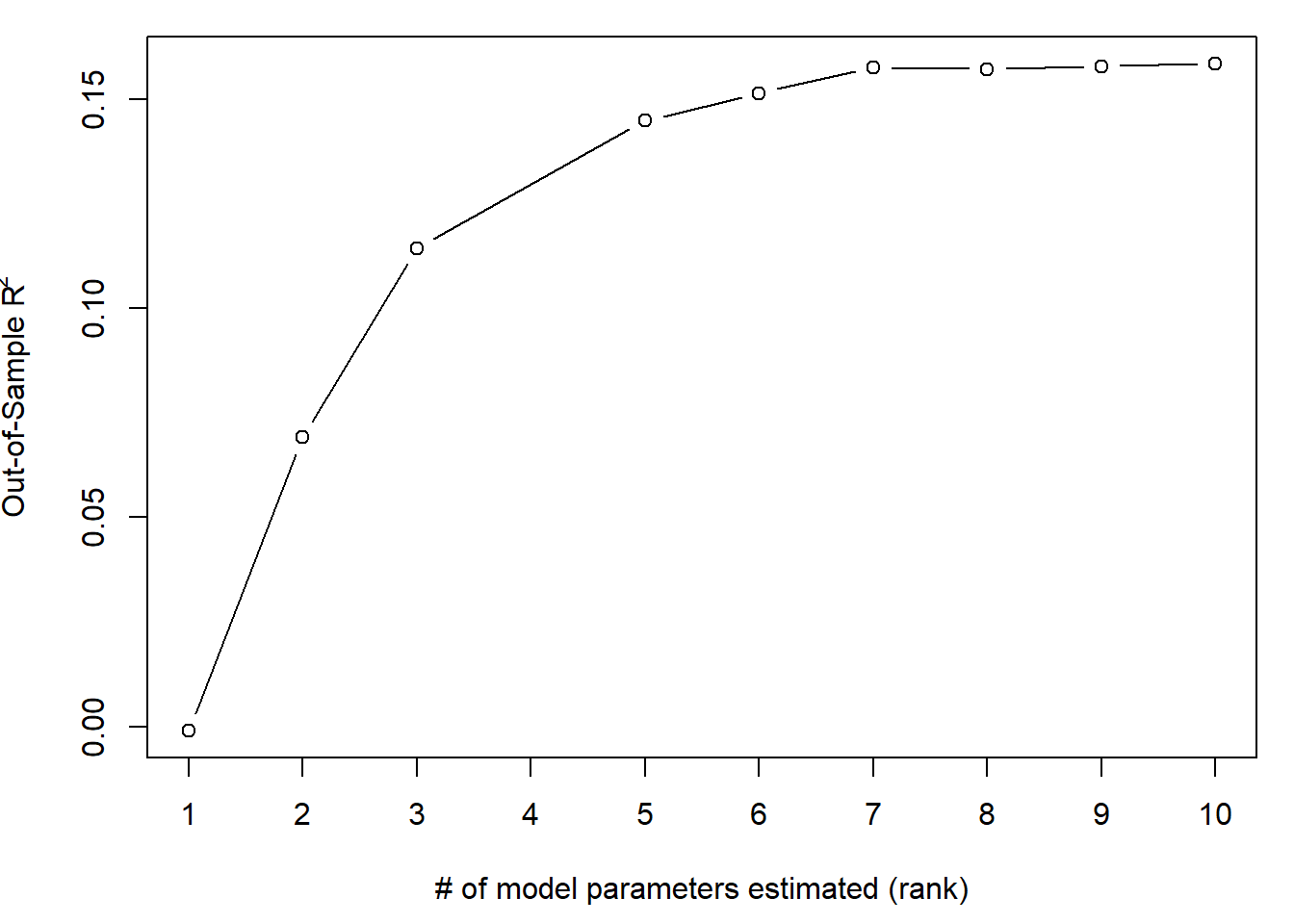

max.idx <- which.max(OOS$R2)

# OOS$rank[max.idx]
cat("Cross Validation Model: ",OOS$rank[max.idx]-1, "coefficients")

## Cross Validation Model:  9 coefficients

ax=c(1:max(OOS$rank))
par(mai=c(.9,.8,.2,.2))
plot(x=OOS$rank, y = OOS$R2, type="b", ylab=expression(paste("Out-of-Sample R"^"2")), xlab="# of model parameters estimated (rank)", xaxt="n")
axis(1, at=ax, labels=ax)
abline(v=OOS$rank[max.idx], lty=3)

model <- fwd.model$keep[["model",max.idx]]

model_full_data<-glm(model$formula, data = bank, family = binomial(link = "logit"))

summary(model_full_data) ## 10-2 = 8 Variables

## 
## Call:
## glm(formula = model$formula, family = binomial(link = "logit"), 
##     data = bank)
## 
## Deviance Residuals: 
##    Min      1Q  Median      3Q     Max  
## -2.327  -0.659  -0.455  -0.268   2.983  
## 
## Coefficients:
##                      Estimate   Std. Error z value             Pr(>|z|)    
## (Intercept)      -3.376667347  0.235940447  -14.31 < 0.0000000000000002 ***
## Age               0.072684500  0.002574758   28.23 < 0.0000000000000002 ***
## IsActiveMember   -1.075352000  0.057666511  -18.65 < 0.0000000000000002 ***
## GeographyGermany  0.774058893  0.067657508   11.44 < 0.0000000000000002 ***
## GeographySpain    0.035864566  0.070625185    0.51                0.612    
## GenderMale       -0.529117847  0.054481703   -9.71 < 0.0000000000000002 ***
## Balance           0.000002653  0.000000514    5.16           0.00000024 ***
## Tenure           -0.015954160  0.009349985   -1.71                0.088 .  
## CreditScore      -0.000668170  0.000280314   -2.38                0.017 *  
## NumOfProducts    -0.100719348  0.047124456   -2.14                0.033 *  
## ---
## Signif. codes:  0 '***' 0.001 '**' 0.01 '*' 0.05 '.' 0.1 ' ' 1
## 
## (Dispersion parameter for binomial family taken to be 1)
## 
##     Null deviance: 10110  on 9999  degrees of freedom
## Residual deviance:  8563  on 9990  degrees of freedom
## AIC: 8583
## 
## Number of Fisher Scoring iterations: 5

Question 4: First non-zero coefficient variable in LASSO?

Run LASSO on the training data.

# all the factor variables
xfactors<- model.matrix(Exited ~ Geography + Gender + HasCrCard + IsActiveMember , data = bank.train)

# remove intercept
xfactors<-xfactors[,-1]

# all continuous variables
x<-as.matrix(data.frame(bank.train$CreditScore, bank.train$Age, bank.train$Tenure, bank.train$Balance, bank.train$NumOfProducts, bank.train$EstimatedSalary, xfactors))                        

lasso_bank <- glmnet(x, y=as.factor(bank.train$Exited), alpha = 1, family = "binomial", nlambda = 100)

par(mai=c(.9,.8,.8,.8))
par(mfrow=c(1,1))
plot(lasso_bank, xvar="lambda", label = TRUE, )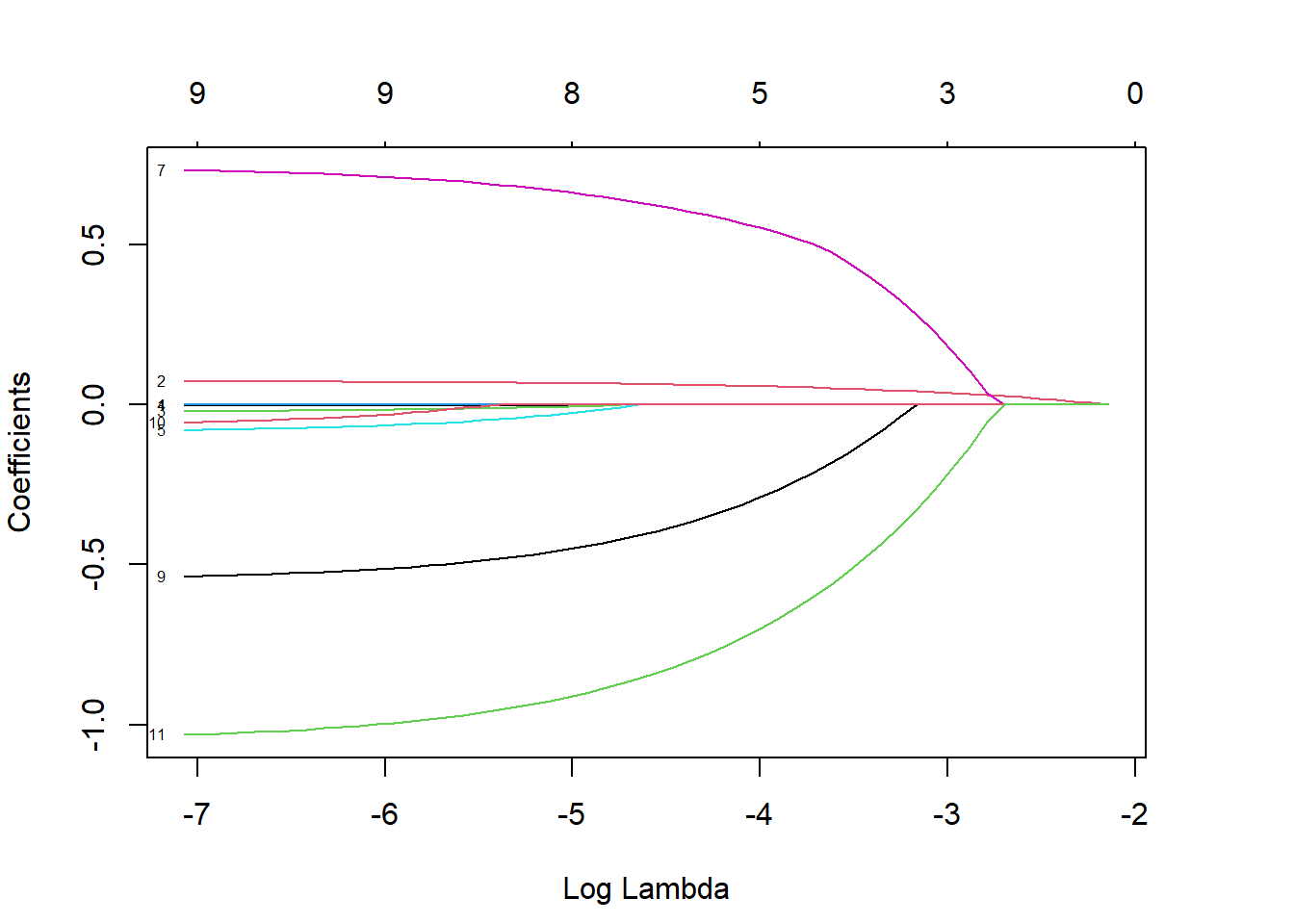

What is the first variable that has a non-zero coefficient as the penalty weight is gradually decreased?

dimnames(x)[2] # Age

## [[1]]
##  [1] "bank.train.CreditScore"     "bank.train.Age"            
##  [3] "bank.train.Tenure"          "bank.train.Balance"        
##  [5] "bank.train.NumOfProducts"   "bank.train.EstimatedSalary"
##  [7] "GeographyGermany"           "GeographySpain"            
##  [9] "GenderMale"                 "HasCrCard"                 
## [11] "IsActiveMember"

## First non-zero coefficient variable:  bank.train.Age  or Age

Question 5: Number of non-zero coefficients in Model

Use cross-validation to tune the penalty weight.

set.seed(19103)
lasso_cv <- cv.glmnet(x, y=bank.train$Exited, family = "binomial", type.measure = "deviance")
plot(lasso_cv)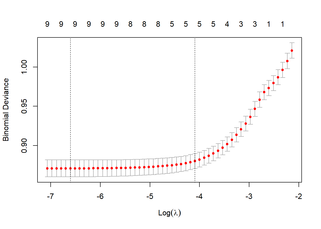

How many non-zero coefficients (excluding the intercept) are there in this model?

## Number of non-zero Coefficients:  9

Question 6: What’s the OOS R2 for the LASSO model?

What’s the OOS R2 for the LASSO model?

Provide your answer with two decimals separated by a dot, not a comma (e.g. 0.12).

cv.glmnet() does k-fold cross-validation for glmnet. Default is nfolds = 10.

## OOS R-Squared:  0.15

Alt: We start by transforming the holdout:

# all the factor variables
xfactors<- model.matrix(Exited ~ Geography + Gender + HasCrCard + IsActiveMember , data = bank.holdout)

# remove intercept
xfactors<-xfactors[,-1]

# all continuous variables
x<-as.matrix(data.frame(bank.holdout$CreditScore, bank.holdout$Age, bank.holdout$Tenure, bank.holdout$Balance, bank.holdout$NumOfProducts, bank.holdout$EstimatedSalary, xfactors))                        

Now we predict:

pred <- predict(lasso_cv, newx=x,  s = "lambda.min", type = "response")
R2(y = bank.holdout$Exited,pred=pred,family="binomial")

## [1] 0.158

Hardcore

set.seed(19103)
n = nrow(bank.train)
K = 10 # # folds
foldid = rep(1:K, each=ceiling(n/K))[sample(1:n)]

OOS=data.frame(R2=rep(NA,K), rank=rep(NA, K))


## pred must be probabilities (0<pred<1) for binomial
deviance <- function(y, pred, family=c("gaussian","binomial")){
    family <- match.arg(family)
    if(family=="gaussian"){
      return( sum( (y-pred)^2 ) )
    }else{
      if(is.factor(y)) y <- as.numeric(y)>1
      return( -2*sum( y*log(pred) + (1-y)*log(1-pred) ) )
    }
  }

## get null devaince too, and return R2
  R2 <- function(y, pred, family=c("gaussian","binomial")){
  fam <- match.arg(family)
  if(fam=="binomial"){
    if(is.factor(y)){ y <- as.numeric(y)>1 }
  }
  dev <- deviance(y, pred, family=fam)
  dev0 <- deviance(y, mean(y), family=fam)
  return(1-dev/dev0)
  }  

for(k in 1:K){
  
  train = which(foldid!=k) 
  
  # train.data conversion
  btrain <- bank.train[train,]
  xfactors<- model.matrix(Exited ~ Geography + Gender + HasCrCard + IsActiveMember, data = btrain)
  xfactors<-xfactors[,-1]
  x <- as.matrix(data.frame(btrain$CreditScore, btrain$Age, btrain$Tenure, btrain$Balance, btrain$NumOfProducts, btrain$EstimatedSalary, xfactors))  
  
   # test.data conversion
  btest <- bank.train[-train,]
  xfactors<- model.matrix(Exited ~ Geography + Gender + HasCrCard + IsActiveMember, data = btest)
  xfactors<-xfactors[,-1]
  xx <- as.matrix(data.frame(btest$CreditScore, btest$Age, btest$Tenure, btest$Balance, btest$NumOfProducts, btest$EstimatedSalary, xfactors))  
  
  #fit regression
  glmnet(x, y=as.factor(btrain$Exited), alpha = 1, family = "binomial", nlambda = 100)
  
  #predict
  pred <- predict(lasso_cv, newx=xx,  s = "lambda.min", type = "response")
  
  #R2
  OOS$R2[k] <- R2(y = btest$Exited,pred=pred,family="binomial")

    # print progress
  cat(k, "  ")
  
}

## 1   2   3   4   5   6   7   8   9   10

round(mean(OOS$R2),2)

## [1] 0.15

  boxplot(OOS[1], data=OOS, main=expression(paste("Out-of-Sample R"^"2")),
        xlab="Model", ylab=expression(paste("R"^"2")))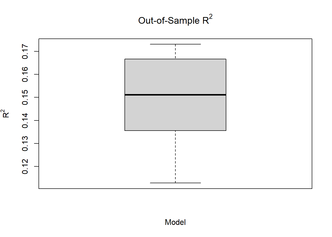

Question 7: How many terminal nodes does the tree have?

Fit a decision tree to the training data with mindev = 0.01.

How many terminal nodes does the tree have?

tree <- tree(as.factor(Exited) ~ ., data=bank.train, mindev=0.01)
summary(tree) # 7

## 
## Classification tree:
## tree(formula = as.factor(Exited) ~ ., data = bank.train, mindev = 0.01)
## Variables actually used in tree construction:
## [1] "Age"            "NumOfProducts"  "IsActiveMember"
## Number of terminal nodes:  7 
## Residual mean deviance:  0.787 = 5510 / 7000 
## Misclassification error rate: 0.164 = 1147 / 7012

par(mfrow=c(1,1))
plot(tree, col=8, lwd=2)
# cex controls the size of the type, 1 is the default.  
# label="yprob" gives the probability
text(tree, label = "yprob", cex=.75, font=2, digits = 2, pretty=0)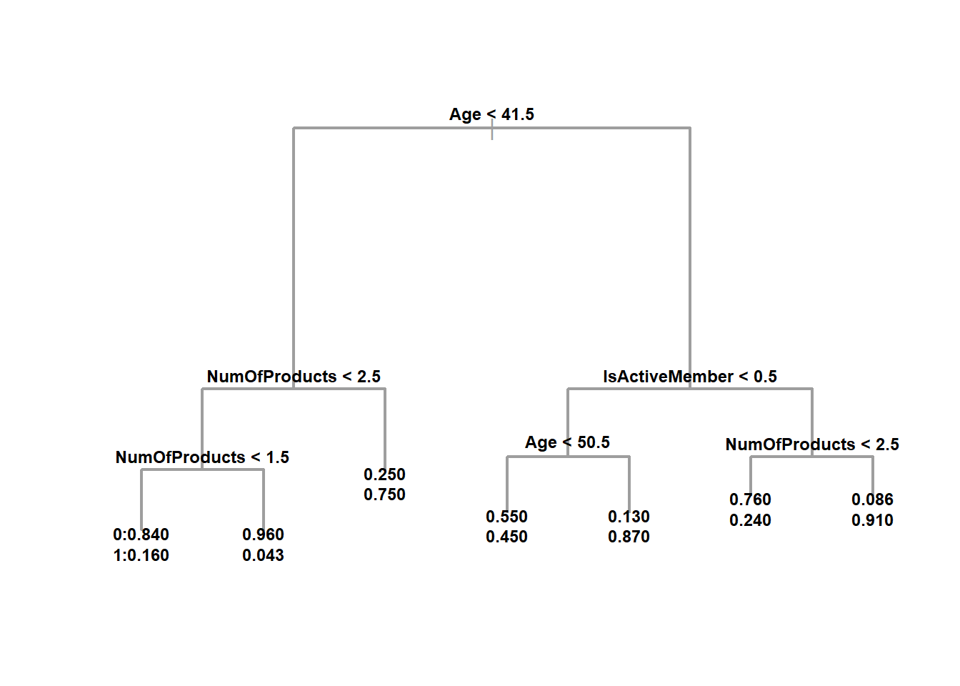

Question 8: Predict Probability

What’s the probability that a 55-year-old German female with 2 products, a 650 credit score, a tenure of 2, a balance of 80.000, a 100.000 salary, no card, not an active member exits?

Provide your answer with two decimals separated by a dot, not a comma (e.g. 0.12).

example <- as.data.frame(cbind(CreditScore = 650, 
                               Geography = "Germany", 
                               Gender = "Female", 
                               Age = 55, 
                               Tenure = 2, 
                               Balance = 80000, 
                               NumOfProducts = 2,
                               IsActiveMember = 0, 
                               HasCrCard = 0, 
                               EstimatedSalary = 100000, 
                               Exited = 1))
example1 <- example %>% 
  mutate(CreditScore = as.integer(CreditScore), 
         Geography = as.factor(Geography), 
         Gender = as.factor(Gender), 
         Age = as.integer(Age), 
         Tenure = as.integer(Tenure), 
         Balance = as.double(Balance), 
         NumOfProducts = as.integer(NumOfProducts),
         IsActiveMember = as.integer(IsActiveMember), 
         HasCrCard = as.integer(HasCrCard), 
         EstimatedSalary = as.double(EstimatedSalary), 
         Exited = as.integer(Exited))

#lets make a prediction for our data. It will create two columns, one with probability for response and no response.
pred_tree <- predict(tree, example1, type = "vector")

## Predicted probability of 0.87 to Exited==1

Question 9: How many terminal nodes does the lowest CV error tree have?

Fit a decision tree with mindev = 0.0001. Use 5 fold cross-validation to prune the tree.

set.seed(19103)
tree_complex <- tree(as.factor(Exited) ~ . , data=bank.train, mindev=0.0001)
summary(tree_complex)

## 
## Classification tree:
## tree(formula = as.factor(Exited) ~ ., data = bank.train, mindev = 0.0001)
## Number of terminal nodes:  553 
## Residual mean deviance:  0.344 = 2220 / 6460 
## Misclassification error rate: 0.0809 = 567 / 7012

## It can be either 7 or 10 depending on whether we define mincut=100 or not

par(mfrow=c(1,1))
par(mai=c(.8,.8,.2,.2))
plot(tree_complex, col=10, lwd=2)
text(tree_complex, cex=.5, label="yprob", font=2, digits = 2, pretty = 0)
title(main="Classification Tree: complex")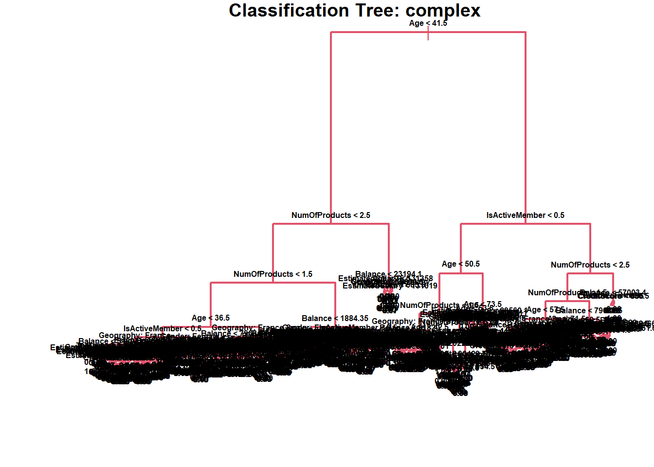

The Model:

set.seed(19103)
cv.tree_complex <- cv.tree(tree_complex, K=5)

#cv.tree_complex <- cv.tree(tree_complex, K=5, FUN = prune.misclass)

How many terminal nodes does the lowest CV error tree have?

par(mfrow=c(1,1))
plot(cv.tree_complex$size, cv.tree_complex$dev, xlab="tree size (complexity)", ylab="Out-of-sample deviance (error)", pch=20) # 7 or 10 Size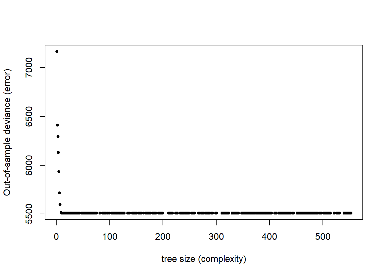

par(mfrow=c(1,2), oma = c(0, 0, 2, 0))
tree_cut <- prune.tree(tree_complex, best=10)
plot(tree_cut, col=10, lwd=2)
text(tree_cut, cex=1, label="yprob", font=2, digits = 2, pretty = 0)
title(main="A pruned tree")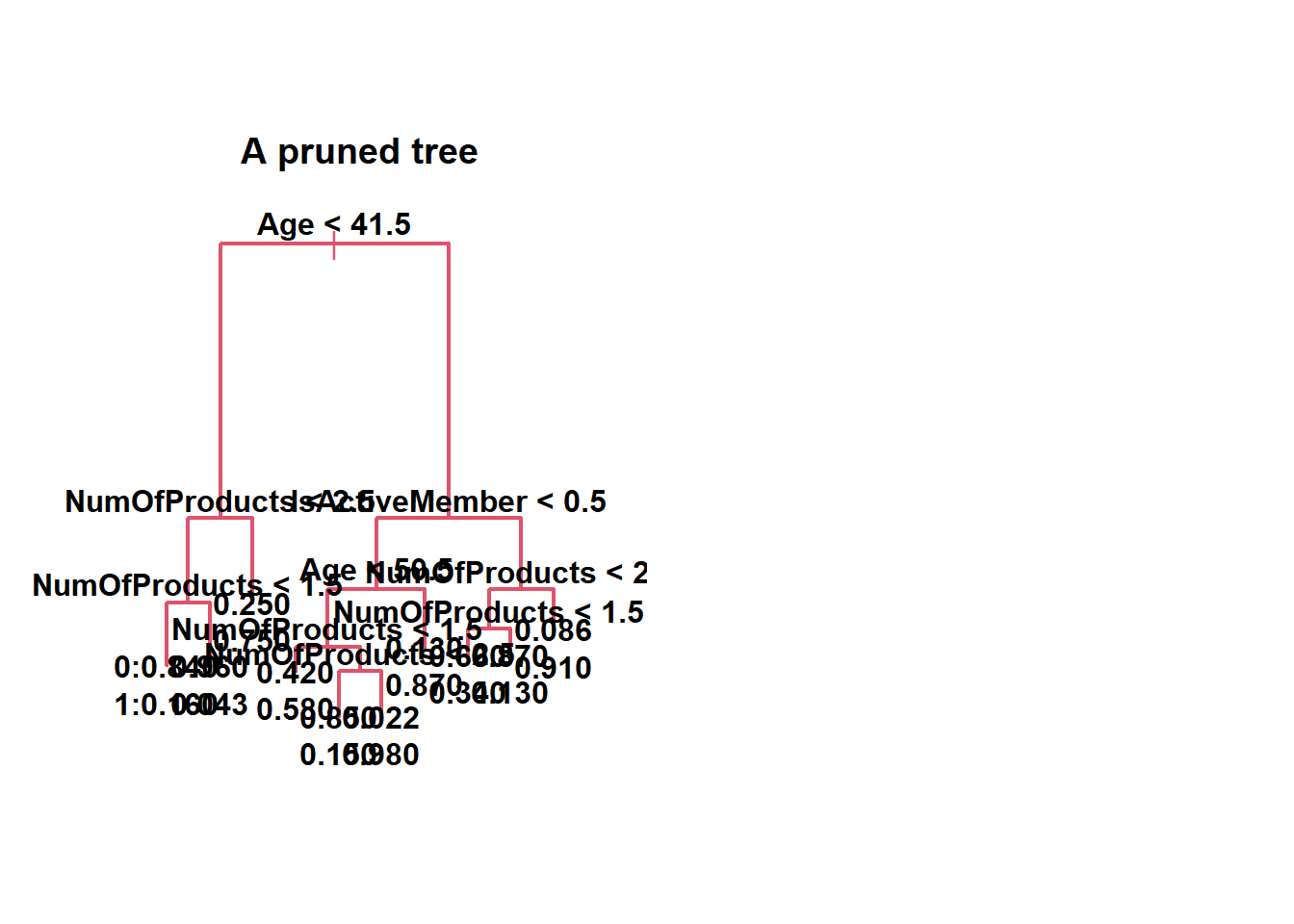

Some Statistic Summary of Pruned Tree:

tree_cut <- prune.tree(tree_complex, best=10) 
summary(tree_cut)

## 
## Classification tree:
## snip.tree(tree = tree_complex, nodes = c(51L, 15L, 50L, 13L, 
## 5L, 24L, 28L, 9L, 29L, 8L))
## Variables actually used in tree construction:
## [1] "Age"            "NumOfProducts"  "IsActiveMember"
## Number of terminal nodes:  10 
## Residual mean deviance:  0.749 = 5250 / 7000 
## Misclassification error rate: 0.148 = 1037 / 7012

Question 10: What is the second most important variable in the random forest?

Use a random forest on the training set with 1000 trees, a minimum node size of 25, importance impurity, probability true, and seed 19103.

set.seed(19103)
bank_rf <- ranger(Exited ~ ., data=bank.train, write.forest=TRUE, num.trees = 1000, min.node.size = 25, importance = "impurity", probability=TRUE, seed = 19103)

par(mfrow=c(1,1))
par(mai=c(.9,.8,.2,.2))
sort(bank_rf$variable.importance, decreasing = TRUE)

##             Age   NumOfProducts         Balance EstimatedSalary     CreditScore 
##           426.8           287.7           159.1           137.9           131.4 
##  IsActiveMember          Tenure       Geography          Gender       HasCrCard 
##            77.8            67.3            49.9            25.5            12.3

barplot(sort(bank_rf$variable.importance, decreasing = TRUE), ylab = "variable importance")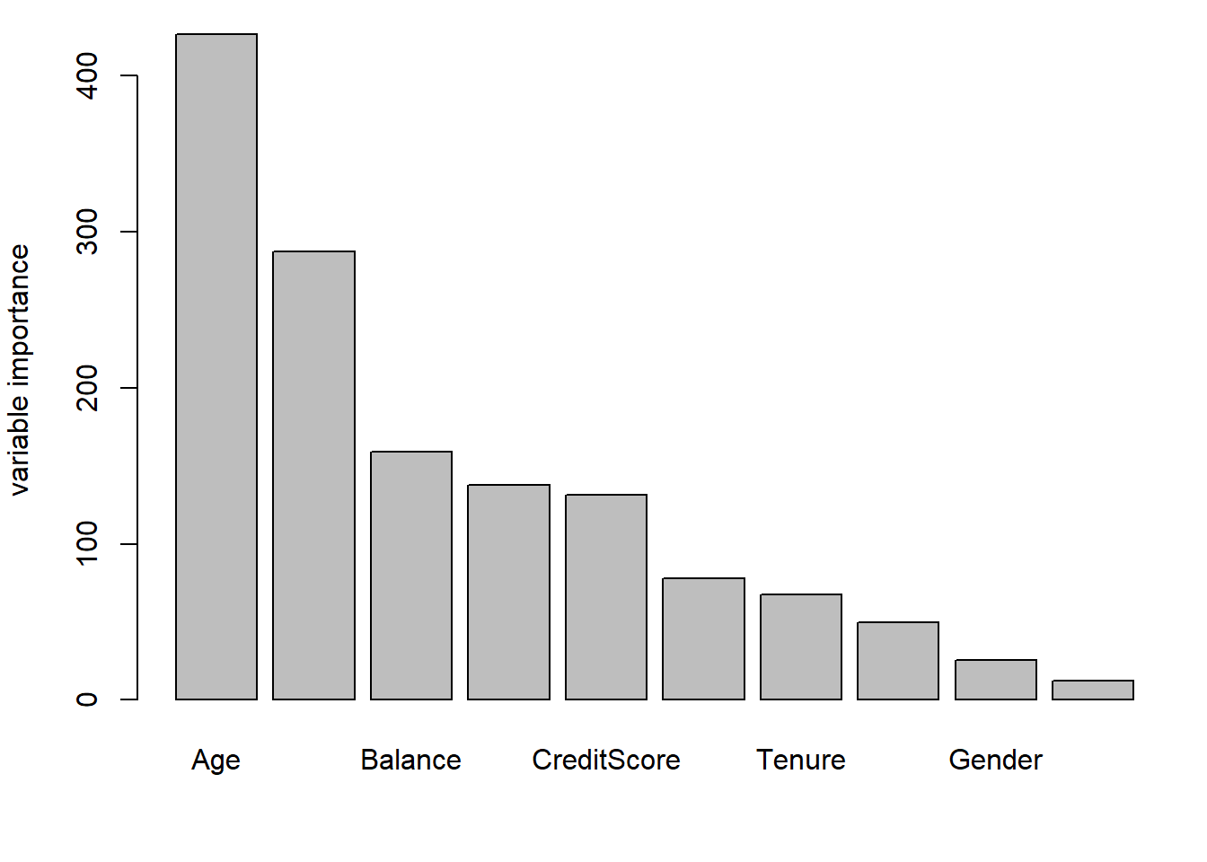

What is the SECOND most important variable in the random forest?

sort(bank_rf$variable.importance, decreasing = TRUE)[2]

## NumOfProducts 
##           288