Assignment 6: CLV - Contractual Settings
Daniel Redel
2022-12-04
Question 1:
Netflix charges 13 euros per month. Variable costs including billing, server capacity, and marketing spending are 2 euros per month. The monthly discount rate is .01. The churn rate is 0.009 per month.
What is the residual lifetime value immediately after renewal (the next payment is due the following month)?
Provide your answer with zero decimals (e.g. 120 or -120).
m <- 13 - 2
d <- 0.01
p <- 1 - 0.009  # churning is the opposite of retention
E(RLV) just the time after the next renewal: \[ E(RLV)=\frac{m(1+d)}{1+d-p}\times \frac{p}{(1+d)} \]
RLV_geo <- m*(1+d)*p/( (1+d-p)*(1+d) )
RLV_geo
## [1] 574Question 2:
Blue Apron is a meal box service, similar to HelloFresh and MarleySpoon. subscribers order several meals a month from the service which are delivered to their homes. Subscribers pay 40 euros a month, where 15 goes to variable costs. The monthly discount rate is .01. Starting with a representative 100 customers in period 0, the number that survives over the following 6 months are given below.
| Months since Joining | Number of Subscribers |
|---|---|
| 0 | 100 |
| 1 | 67 |
| 2 | 50 |
| 3 | 41 |
| 4 | 34 |
| 5 | 31 |
| 6 | 28 |
How much higher is the actual retention rate at 6 months than at 1 month?
Provide your answer with two decimals separated by a dot, not a comma (e.g. 0.12).
First, we create the dataset:
active_subs=c(100,
              67,
              50,
              41,
              34,
              31,
              28)
data <- cbind(0:6, active_subs)
colnames(data) <- c("Period", "Active Subscribers")
data %>%
  kbl() %>%
kable_styling()| Period | Active Subscribers |
|---|---|
| 0 | 100 |
| 1 | 67 |
| 2 | 50 |
| 3 | 41 |
| 4 | 34 |
| 5 | 31 |
| 6 | 28 |
\[ r(t) = P(T>t \mid T>t-1) = \frac{S(t)}{S(t-1)} \] Survivor Function:
lost <- -diff(active_subs)

S <- active_subs[1:11]/active_subs[1] # Survivor Function

data <- cbind(data, S)
## Warning in cbind(data, S): number of rows of result is not a multiple of vector length (arg 2)Retention Rate:
r <- S[2:11]/S[1:10] # DEFINITION

data <- cbind(data, c(NA,r))
## Warning in cbind(data, c(NA, r)): number of rows of result is not a multiple of vector length (arg 2)colnames(data)[[4]] <- "r"
data %>%
kbl() %>%
kable_styling()| Period | Active Subscribers | S | r |
|---|---|---|---|
| 0 | 100 | 1.00 | NA |
| 1 | 67 | 0.67 | 0.670 |
| 2 | 50 | 0.50 | 0.746 |
| 3 | 41 | 0.41 | 0.820 |
| 4 | 34 | 0.34 | 0.829 |
| 5 | 31 | 0.31 | 0.912 |
| 6 | 28 | 0.28 | 0.903 |
How much higher is the actual retention rate at 6 months than at 1 month? Answer:
round(0.903-0.670,2)## [1] 0.23Retention Rate Plot:
par(mai=c(.9,.8,.2,.2))
plot(0:10, S, type="b",ylab="Survival Function S(t)", xlab="Period",ylim=par("yaxp")[1:2]) 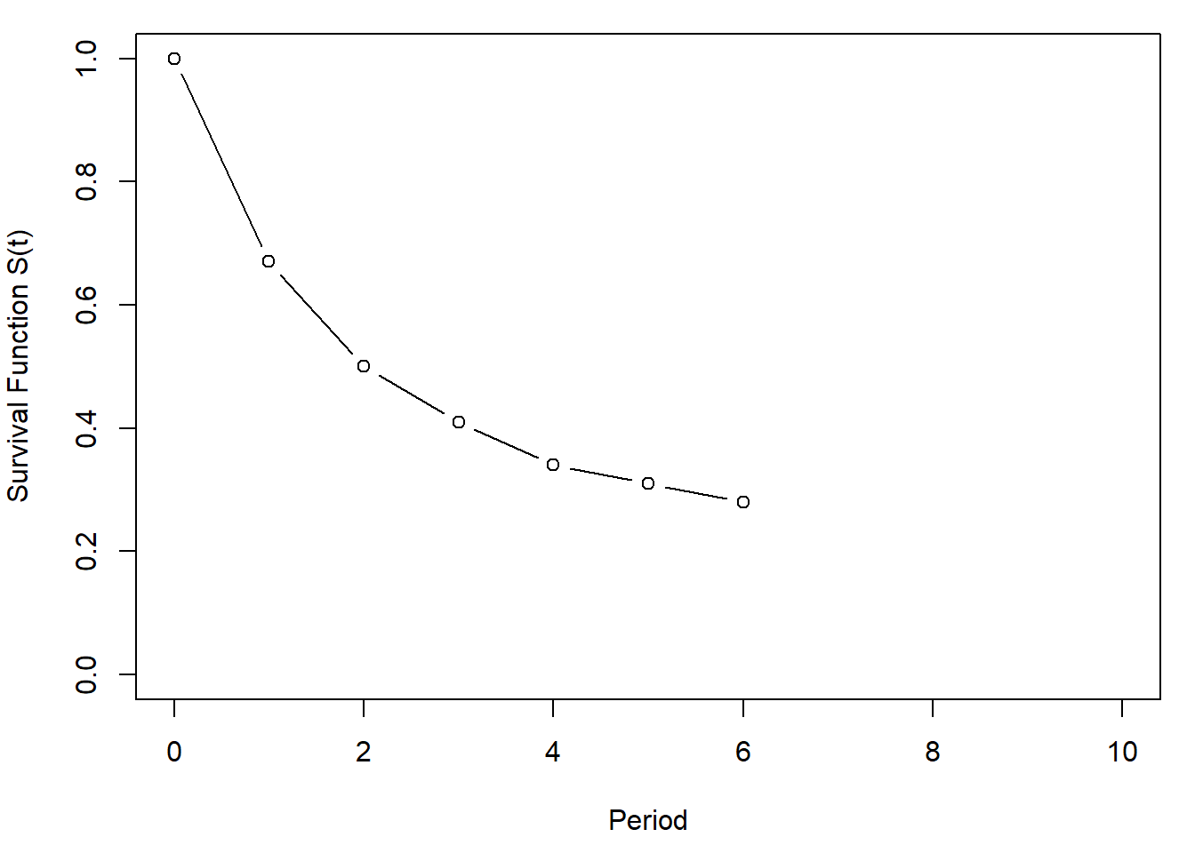
par(mai=c(.9,.8,.2,.2))
plot(1:10, r, type="b",ylab="retention rate r(t)", xlab="Period",ylim=par("yaxp")[1:2]) 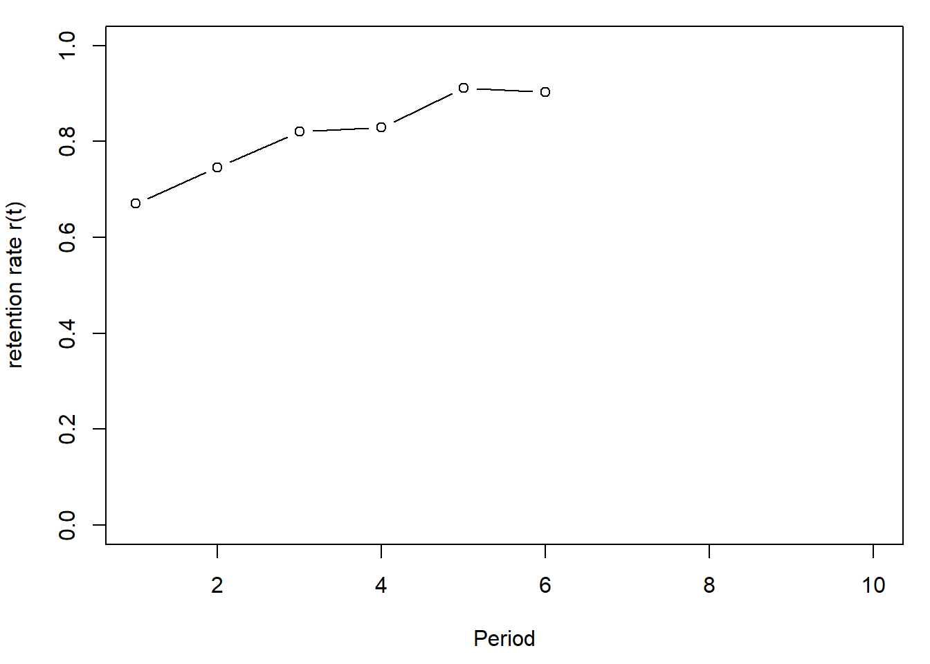
Question 3:
Fit the Beta-Geometric model to the retention data using only data from the beginning until (and including) 4 months since joining. For your estimation use starting values a = 1 and b = 1.
What are the estimates of a and b?
Provide your answer with three decimals separated by a dot, not a comma (e.g. 0.123).
r_sBG=function(a,b,t){
    (b+t-1)/(a+b+t-1)
}

lost <- -diff(active_subs[1:5])
active <- active_subs[1:5][-1]
loop.lik <- function(params) {
a <- params[1]
b <- params[2]
ll <- 0
for (i in 1:length(lost)) {
ll <- ll+lost[i]*log(beta(a+1,b+i-1)/beta(a,b))
}
ll <- ll+active[i]*log(beta(a,b+i)/beta(a,b))
return(-ll) #return the negative of the function to maximize likelihood
}
#find parameters for a and b with optim
sBG <- optim(par=c(1,1),loop.lik)
a<-sBG$par[1]
b<-sBG$par[2]
a## [1] 0.955b## [1] 1.93#calculate retention using model parameters
t <- 1:length(active)
r_pred <- r_sBG(a,b,t)
S_pred <- c(1,cumprod(r_pred)) # predicted survivor functionr <- S[2:11]/S[1:10] # DEFINITION
# plot actual and predicted retention rate
par(mfrow=c(1,1))
plot(t,r_pred,ylab="retention rate",xlab="period",type="b", xaxt="none", ylim = c(.55,1))
lines(t, r[1:4], type="b", col="blue")
axis(1, seq(0,10,1))
legend('right',legend=c("sBG", "actual"),col=c("black","blue"), pch=c(1,1))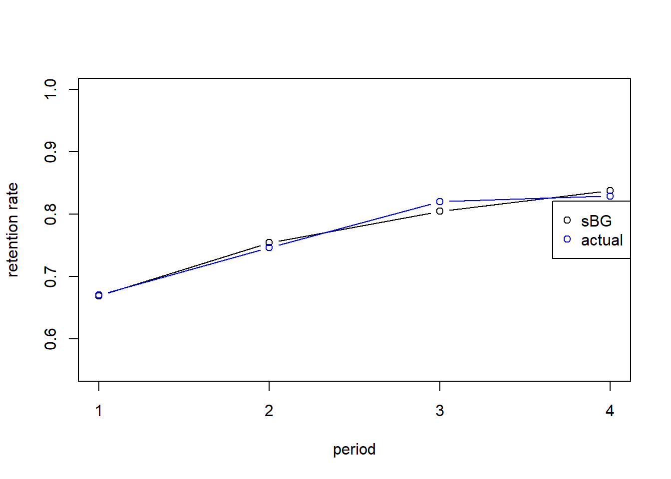
Question 4:
Our holdout sample is everything after period 4. For the model fit in Q3, calculate the mean absolute error of the holdout retention rate.
Provide your answer with two decimals separated by a dot, not a comma (e.g. 0.12).
First, we predict the retention rate in the holdout sample:
r_sBG=function(a,b,t){
    (b+t-1)/(a+b+t-1)
}

t <- 1:length(active_subs[-1])
r_pred <- r_sBG(a,b,t)
We now evaluate using MAE Criteria:
round(mae(r[5:6], r_pred[5:6]),2)## [1] 0.04#Dataset
data.fit <- cbind(pred=r_pred, actual=r[1:6])
data.fit %>%
kbl() %>%
kable_styling()| pred | actual |
|---|---|
| 0.669 | 0.670 |
| 0.754 | 0.746 |
| 0.805 | 0.820 |
| 0.838 | 0.829 |
| 0.861 | 0.912 |
| 0.879 | 0.903 |
par(mfrow=c(1,1))
plot(t,r_pred,ylab="retention rate",xlab="period",type="b", xaxt="none", ylim = c(.55,1))
lines(t, r[1:6], type="b", col="blue")
axis(1, seq(0,10,1))
legend('right',legend=c("sBG", "actual"),col=c("black","blue"), pch=c(1,1))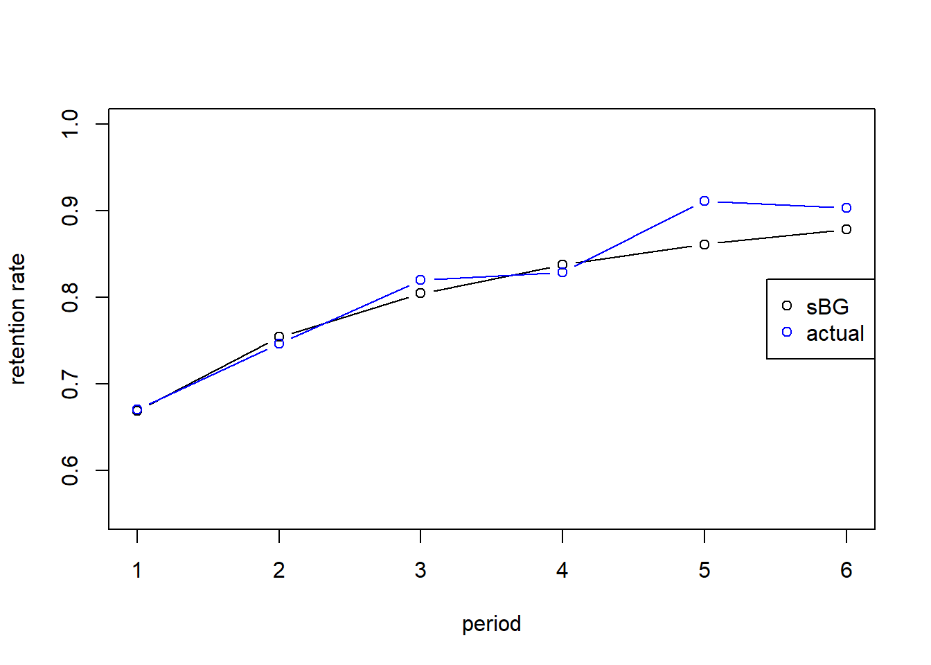
Question 5:
According to your model fit in Q3, what percentage of customers will be active one year after the first signup?
Provide your answer with two decimals without the percent sign separated by a dot, not a comma (e.g. 0.12).
t <- 1:12
r_pred <- r_sBG(a,b,t)

S_pred <- c(1,cumprod(r_pred))
S_pred[13]
## [1] 0.15cbind(retention=c(1,r_pred), survivor=S_pred) %>%
kbl() %>%
kable_styling()| retention | survivor |
|---|---|
| 1.000 | 1.000 |
| 0.669 | 0.669 |
| 0.754 | 0.504 |
| 0.805 | 0.406 |
| 0.838 | 0.340 |
| 0.861 | 0.293 |
| 0.879 | 0.257 |
| 0.893 | 0.230 |
| 0.903 | 0.208 |
| 0.912 | 0.189 |
| 0.920 | 0.174 |
| 0.926 | 0.161 |
| 0.931 | 0.150 |
Question 6:
Up to how much would Blue Apron spend to rescue a customer who has renewed once, immediately after that first renewal?
Use 200 time periods for your simulation and round to whole euros.
Provide your answer with zero decimals (e.g. 120 or -120).
Let’s try this out for someone who has renewed \(\tau=1\) times:
tau <- 1
m <- 40 - 15
d <- 0.01
t <- seq(1,tau+200)

r_pred <- r_sBG(a,b,t)
S_pred <- cumprod(r_pred)

S_shift <- S_pred[(tau+1):length(S_pred)]  # survival function from tau + 1 until T

dis <- 1/(1+d)^(t(1:200)-1) # discount rate

RLV_sBG <- sum(m*S_shift/S_pred[tau]*dis)  # sum of margin x S(tau + t)/ S(tau) x discount
RLV_sBG
## [1] 229Question 7:
How much more is that amount (in Q6) than the customer lifetime value for a new customer?
Provide your answer with zero decimals (e.g. 120 or -120).
t <- seq(1,200) # time periods
r_pred <- r_sBG(a,b,t) # predicted retention rate
S_pred <- c(1,cumprod(r_pred)[1:199]) # predicted survivor function

dis <- 1/(1+d)^(t-1) # discount factor, first term is present so no discounting

CLV_sBG <- sum(m*S_pred*dis) # the sum of margin x survivor x discount factor

RLV_sBG - CLV_sBG
## [1] 37.3