Assignment 1: Test & Roll

Case 1

A company wants to calculate the value of testing. They have a margin of 25, a marketing cost of 1, and a total customer base of 100.000. Their sample is 5.000 customers. In the past, campaigns have either been a success, with a response rate of 0.05, or a failure, with a response rate of 0.03. Historically, 60% of past mailings have been a failure.

1. What is the expected profit if the company launches the marketing campaign without doing a test?

Our Parameters:

N = 100000 # Customer base
n = 5000 # number in test sample
c = 1 # cost
m = 25 # margin

# Success (Prob=0.4)
p_s = 0.05
# Failure (Prob=0.6)
p_f = 0.03

We can use the following formula:

\[ \Pr(\text{success})\times[N(p_sm-c)] + \Pr(\text{failure})\times[N(p_fm-c)] \]

profit_notest = N*((0.4)*((p_s*m-c))+(0.6)*((p_f*m-c)))

## Expected Profit without doing the test: -$ 5000

2. What is the value of doing the test?

\[ \Pr(\text{success})\times[N(p_sm-c)] + \Pr(\text{failure})\times[n(p_fm-c)] - 0 \]

profit_test <- (0.4)*((N)*(p_s*m-c))+(0.6)*((n)*(p_f*m-c))-0 

## Expected Profit if we run the test: $ 9250

Case 2

A company ran an A/B test and got conversion rates of 30.7% and 32.4% for versions A and B. Assume flat priors and 1000 people in each group; use 10000 draws and set seed at 19312.

set.seed(19312)

n <- 1000 # obs for A
n <- 1000 # obs for B

# Conversion Rates
ybar_A <- 30.7*0.01
ybar_B <- 32.4*0.01

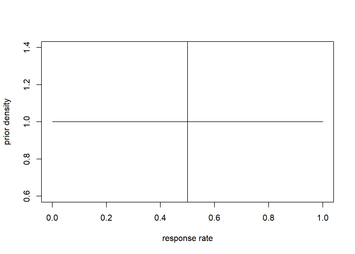
From the prior, \(a_{A,B}=1\) and \(b_{A,B}=1\).

prior_a = 1
prior_b = 1

xx <- seq(0, 1,length=100)
plot(xx, y=dbeta(xx, shape1=prior_a, shape2 = prior_b), 
     type="l", col="black", xlab="response rate", ylab="prior density")
abline(v=prior_a/(prior_a+prior_b))

3. What’s the probability that the posterior mean response rate of B is larger than that of A?

Provide your answer with three decimals separated by a dot, not a comma (e.g. 0.123).

We start estimating the posterior mean response rate. Recall that:

\[ E[p]=\frac{a}{a+b} \]

#posterior distribution 
postA_a = prior_a + n*ybar_A
postA_b = prior_b + n - n*ybar_A
postB_a = prior_a + n*ybar_B
postB_b = prior_b + n - n*ybar_B

## Posterior Response Rate of A 0.31

## Posterior Response Rate of B 0.32

We now can get the probability that the response rate of B is larger than A, \(\Pr(p_A<p_B)\):

set.seed(19312)
B <- 10000
post_draws_A <- rbeta(B,postA_a,postA_b)
post_draws_B <- rbeta(B,postB_a,postB_b)
prob = sum(post_draws_B>post_draws_A)/B

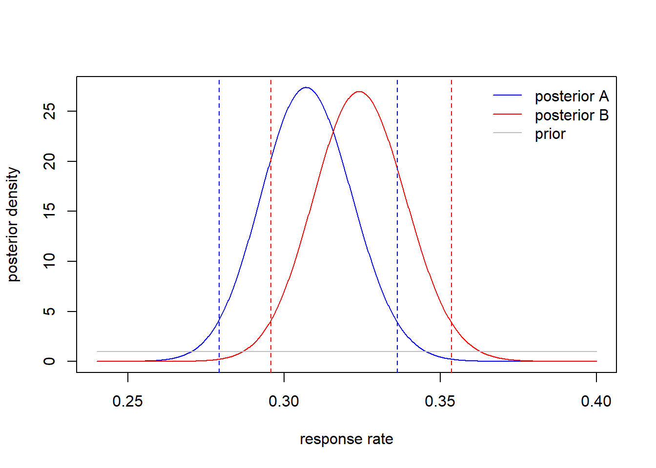
## Probability that B>A is 0.795

The 95% Confidence Intervals:

ci95_A <- qbeta(c(0.025, 0.975), shape1=postA_a, shape2 = postA_b) # CI for A
ci95_B <- qbeta(c(0.025, 0.975), shape1=postB_a, shape2 = postB_b) # CI for B

## [ 0.28 0.34 ]

## [ 0.3 0.35 ]

Finally, we plot our results:

xx=seq(0.24,0.4,length=1000)

plot(xx, y=dbeta(xx, shape1=postA_a, shape2 = postA_b), 
     type="l", col="blue", xlab="response rate", ylab="posterior density")
lines(xx, y=dbeta(xx, shape1=postB_a, shape2 = postB_b), 
     type="l", col="red", xlab="response rate", ylab="posterior density")
lines(xx, y=dbeta(xx, shape1=prior_a, shape2 = prior_b), type="l", col="gray")
legend("topright", col=c("blue", "red", "grey"), legend=c("posterior A", "posterior B", "prior"), bty="n", lty=1)
text(x = .34,y= 58, paste("P(m_A < m_B) = ", round(prob,3)))
abline(v=ci95_A, col="blue", lty=2)
abline(v=ci95_B, col="red", lty=2)

Case 3

A company with 50.000 customers wants to run an A/B test of two different versions of a website. The outcome they want to test is time on site, rolling out whichever version leads to people spending more time there. The average amount of time spent is 5 minutes and the standard deviation of time spent is about 2. The mean across treatments varies with a standard deviation of 0.5.

4. How many people should there be in each test group?

\[ n_A^*=n_B^*=\sqrt{\frac{N}{4}\left(\frac{s}{\sigma}\right)^2+\left(\frac{3}{4}\left( \frac{s}{\sigma} \right)^2 \right)^2 }-\frac{3}{4}\left( \frac{s}{\sigma} \right)^2 \]

set.seed(19312)
N <- 50000 # available population
s <- 2  # how variable the profit is from one customer to another.
sigma <- 0.5 # range of expected conversation rates across previous treatments
mu <- 5  # NOT RELEVANT: average conversion rate across previous treatments

## Optimal Test Sample Size: 435